
Building Load Model Forecasting from AMI Data
How to use a model fitted to AMI data to do load forecasting.
In a previous post I described how to fit a discrete linear time-invariant (LTI) dynamic model to AMI or SCADA data from loads. In this post I want to extend that method to the problem of load forecasting. The idea is pretty simple, if we can use an LTI model to predict the next hour, then we can use it to predict an arbitrary number of hours in the future, with the expectation that the further ahead the prediction, the less accurate it is.
Just as a reminder, the LTI model is presented in $z$-domain in the form
\[\frac{P(z)}{T(z)} = \frac{b_0+b_1z^{-1}+\cdots+b_Mz^{-M}}{1+a_1z^{-1}+\cdots+a_Nz^{-N}} \qquad \mathrm{where} ~ N \ge M.\]If we have $K$ samples at the regular interval $t_s$ for $T$ and $P$, then we define the matrix
\[\mathbf{M} = \begin{bmatrix} \mathbf{P}_1 & \cdots & \mathbf{P}_N & \mathbf{T}_0 & \cdots & \mathbf{T}_M \end{bmatrix}\]where
\[\mathbf{T}_k = \begin{bmatrix} T(k) & \cdots & T(K-N+k-1) \end{bmatrix}^\mathrm{T},\] \[\mathbf{P}_k = \begin{bmatrix} P(k) & \cdots & P(K-N+k-1) \end{bmatrix}^\mathrm{T},\]and the vector
\[\mathbf{b} = \begin{bmatrix} \mathbf{P}_0 & \cdots & \mathbf{P}_{-h} \end{bmatrix}.\]where $h$ is the number of hours being forecasted.
We then evaluate $\mathbf{x} = ( \mathbf{M}^T \mathbf{M} )^{-1} \mathbf{M}^T \mathbf{b}$ to obtain the coefficients of the discrete-time transfer function. This is the forecasting model for $h$ hours. The variation we have introduced is essentially the original vector $\mathbf{b}$ copied $h$ times and shifted by one hour for each column.
We will use the same example as the original post, and use this extension to perform a 96 hour load forecast. First, we import the training data:
from pandas import read_csv
data = read_csv('data.csv',index_col=['t'],parse_dates=[0])
print(data)
                                 P     T
t
2020-07-01 01:00:00-07:00  3.61584  15.2
2020-07-01 02:00:00-07:00  3.96148  14.2
2020-07-01 03:00:00-07:00  4.60248  13.2
2020-07-01 04:00:00-07:00  5.39665  12.1
2020-07-01 05:00:00-07:00  6.13824  11.1
...                            ...   ...
2020-07-31 20:00:00-07:00  4.82946  16.7
2020-07-31 21:00:00-07:00  4.22882  16.3
2020-07-31 22:00:00-07:00  3.78543  16.0
2020-07-31 23:00:00-07:00  3.59467  15.9
2020-08-01 00:00:00-07:00  3.57846  15.7

[744 rows x 2 columns]
We process the data and solve the model fit problem using a high-order thermal model for the building
from numpy import array, hstack
from numpy.linalg import solve

inputs = ['T']
output = 'P'
K = 25 # model order
H = 24 # forecast hours

X = array(data[inputs])
Y = array(data[[output]])
L = len(Y)
M = hstack([hstack([Y[n:L-K+n-H+1] for n in range(K)]),
            hstack([X[n:L-K+n-H+1] for n in range(K+1)])])
Mt = M.transpose()
b = hstack([Y[K+n:L+n-H+1] for n in range(H)])
x = solve(Mt@M,Mt@b)
This gives us $x$ which is the $H$-hour forecasting model based on a $K$-th order dynamic load model.
Validation
To validate the performance of the model, we use data that was not included in the original dataset.
test = pd.read_csv('test.csv',index_col=['t'],parse_dates=[0])
print(test)
                                 P     T
t
2020-08-01 01:00:00-07:00  3.55169  15.6
2020-08-01 02:00:00-07:00  3.56701  15.4
2020-08-01 03:00:00-07:00  3.66880  15.3
2020-08-01 04:00:00-07:00  3.98450  15.1
2020-08-01 05:00:00-07:00  4.29065  15.0
...                            ...   ...
2020-08-07 20:00:00-07:00  4.73422  16.1
2020-08-07 21:00:00-07:00  4.48835  15.6
2020-08-07 22:00:00-07:00  4.01017  15.0
2020-08-07 23:00:00-07:00  3.87611  14.4
2020-08-08 00:00:00-07:00  3.89687  13.3

[168 rows x 2 columns]
We can use the matrix $M$ for the test data to visualize the performance of the result.
X = array(test[inputs])
Y = array(test[[output]])
L = len(Y)
M = hstack([hstack([Y[n:L-K+n-H+1] for n in range(K)]),
hstack([X[n:L-K+n-H+1] for n in range(K+1)])])
import matplotlib.pyplot as plt
plt.subplots(2,2,figsize=(15,10))
isdst = 1
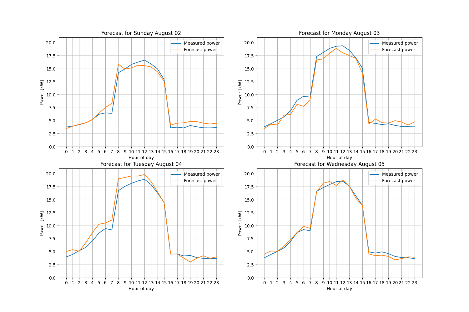
for t in range(0,96,24):
tt = [str((h.hour-1-isdst)%24) for h in test.index[K+t:K+H+t]]
plt.subplot(2,2,int(t/24)+1)
plt.plot(tt,Y[K+t:K+H+t],label='Measured power')
plt.plot(tt,(M@x)[t].transpose(),label='Forecast power')
plt.grid()
plt.ylim([0,21])
plt.xlabel('Hour of day')
plt.ylabel('Power [kW]')
plt.legend()
plt.title(f"Forecast for {test.index[t+K].strftime('%A %B %d')}")
plt.savefig(f"../../images/2023-02-15-Figure_1.png")
plt.show()
from matplotlib.patches import Rectangle
plt.subplots(2,2,figsize=(15,10))
NL="\n"
for t in range(0,96,24):
    err = ((M@x)[t]/Y[K+t:K+H+t].transpose()[0] - 1)*100
    tt = [str((h.hour-1-isdst)%24) for h in test.index[K+t:K+H+t]]
    plt.subplot(2,2,int(t/24)+1)
    plt.gca().add_patch(Rectangle([float(tt[0]),err.mean()-err.std()],23.0,2*err.std(),facecolor='lightgrey'))
    plt.plot(tt,err,label=f"Forecast error")
    plt.plot([tt[0],tt[-1]],[err.mean(),err.mean()],"--k",label="Mean and stdev")
    plt.ylim([-33,33])
    plt.grid()
    plt.xlabel('Hour of day')
    plt.ylabel('Error [%]')
    plt.title(test.index[K+1+t].strftime('Forecast error for %A %B %d'))
    plt.legend()
plt.savefig(f"../../images/2023-02-15-Figure_2.png")
plt.show()
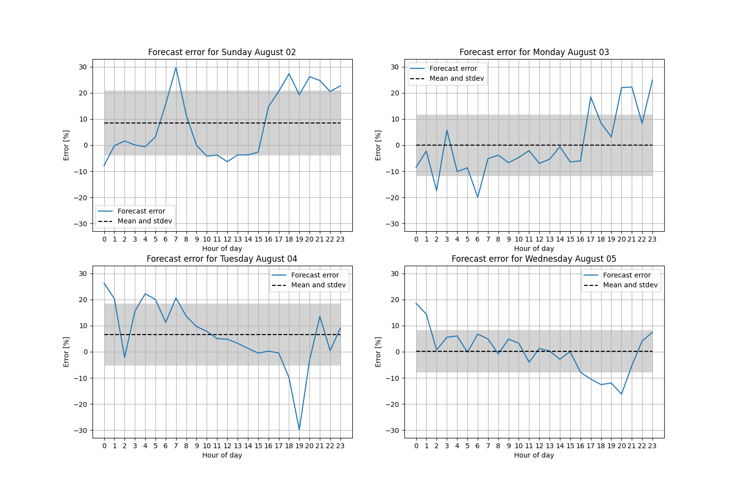
We can see that the forecasts are generally satisfactory for such a simple model, although the forecast for a similar daytype (i.e., weekday, weekend) is better than for a different daytype.