
Notes on demand response dynamics and load forecasting
“Prediction is very difficult, especially about the future”
There are many variant to this Neils Bohr quote, but they all convey the same idea, and it quite relevant to load forecasting. The load forecasting problem has become even more difficult when the advent of price-responsive loads such as those emerging in transactive energy systems. This post is about my attempts to model some of the dynamic behavior we see in loads and which should be included in load forecasting models.
In transactive energy systems, the sigmoid demand curve at equilibrium has been derived from first principles [1] to describe the expected shape of the demand function. It is generally presented as a logistic function based on the random utility model [2] and has the form
\[Q(P) = \frac{Q_R}{1+e^{ 2 \eta_D \left( 1-\frac{P}{\hat P} \right) }} + Q_U\]where $P$ is the price, $Q(P)$ is the quantity at the price $P$, $Q_R$ is the total demand that is responsive to the price, $Q_U$ is the total demand is not response to price, $\hat P$ is the most probable price, and $\eta_D$ is the demand elasticity at equilibrium. An example is shown in Figure 1.
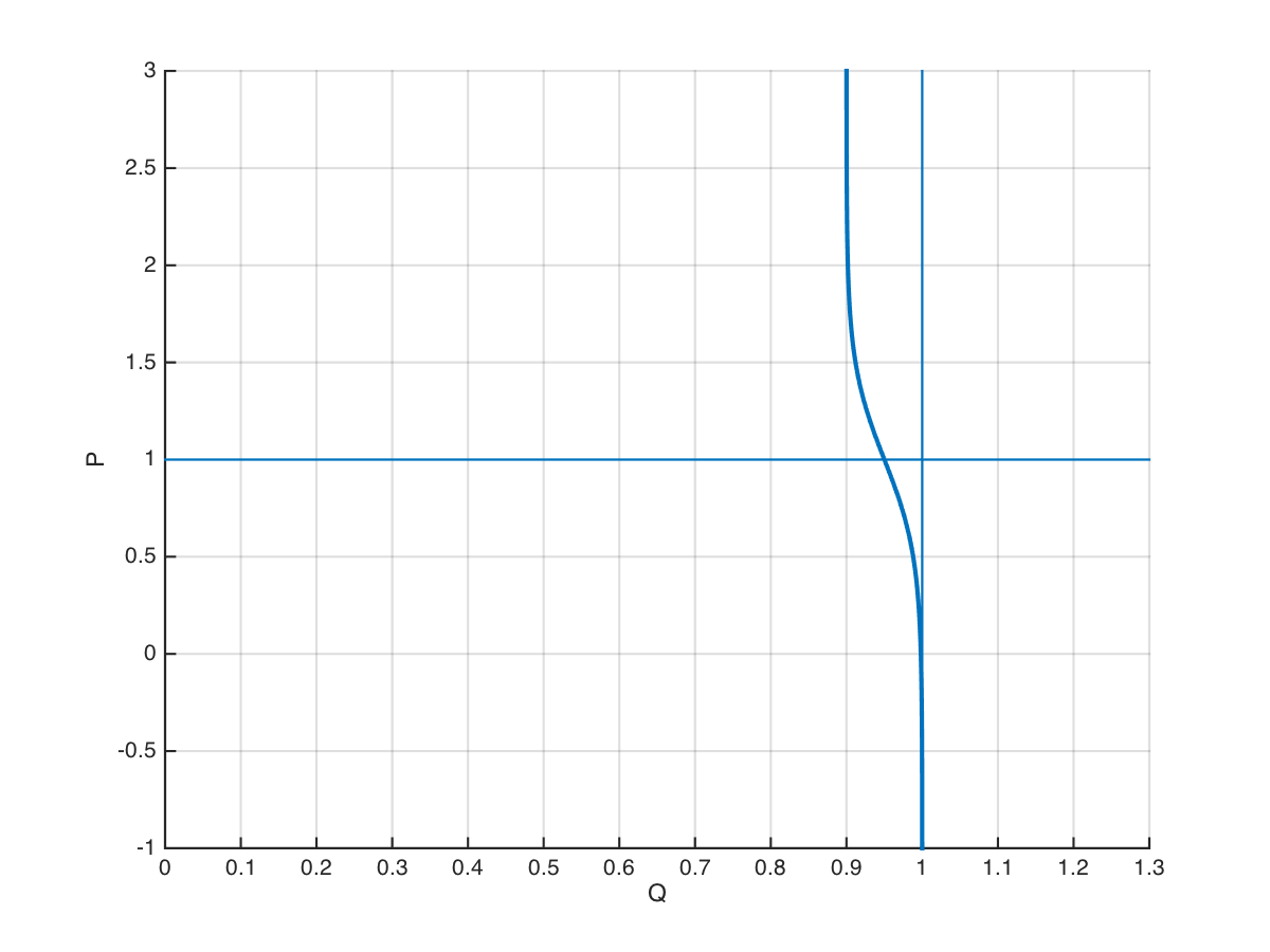
Figure 1: Logistic demand function at 50% duty cycle
The equilibrium model assumes that the duty cycle of the load is 0.5 and when it is not, the model must be extended to account for the natural imbalance between loads that are on and loads that are off. One simple method is to directly weight the state probabilities using the duty cycle $0 \le D \le1$ such that
\[Q(P) = \frac{DQ_R}{D+(1-D)e^{2\eta_D \left( 1-\frac{P}{\hat P} \right)}} + Q_U \qquad (1)\]Although this result has not been compared to field data, it presents the correct behavior and can be justified well in terms of the same state statistics used to derive the original logistic function. The low and high load examples are shown in Figure 1. In the extreme case, the extended model exhibits the correct behavior, as shown in Figure 2.
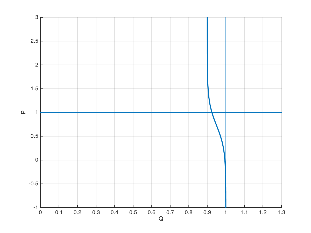
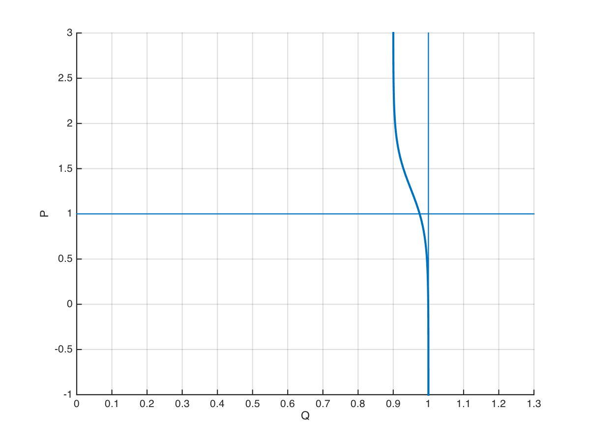
Figure 2: Logistic demand function at 25% duty cycle (top) and 75% duty cycle (bottom)
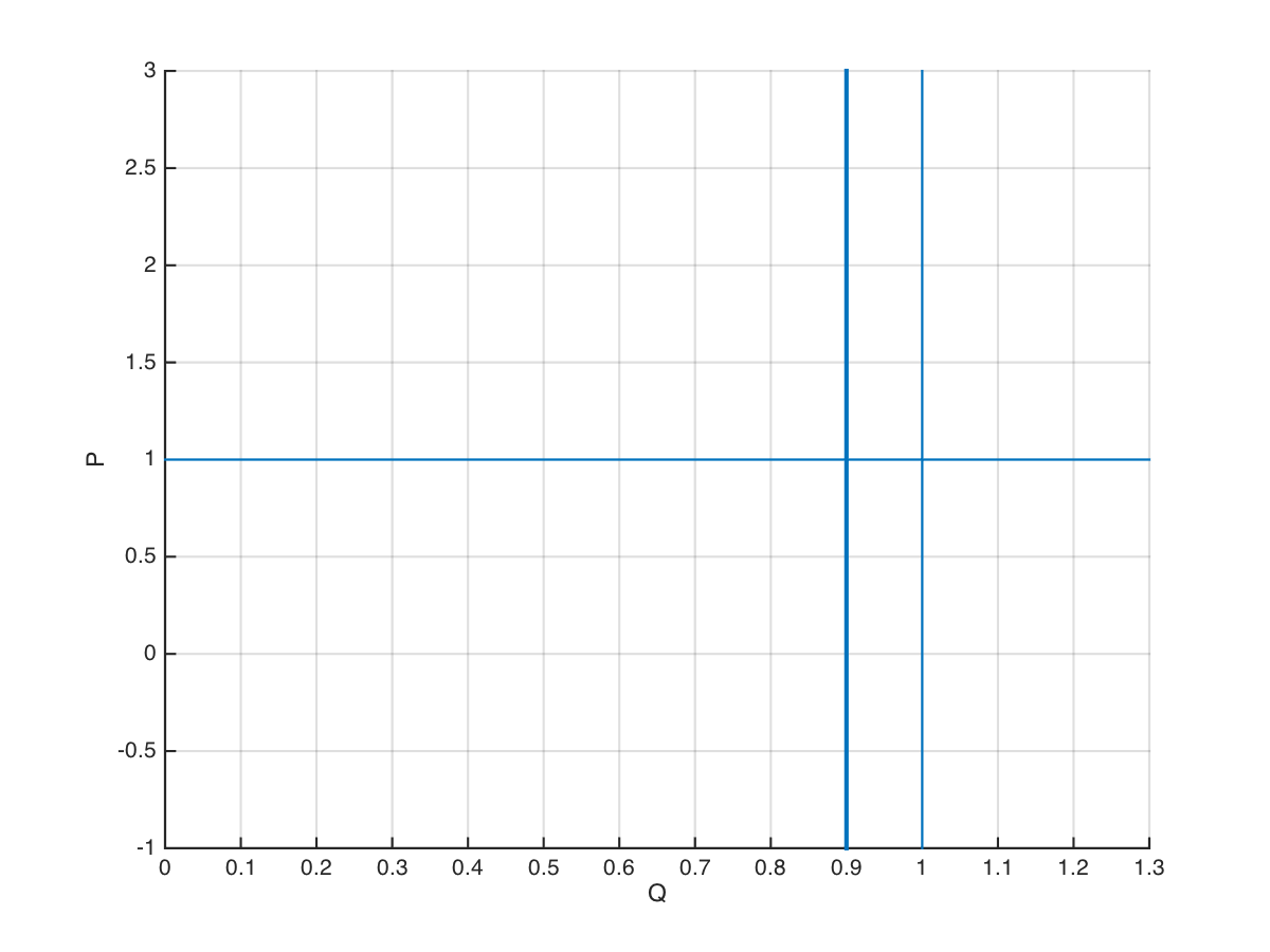
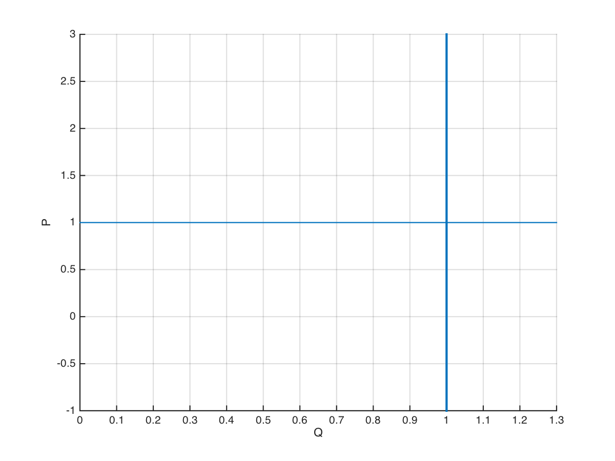
Figure 3: Logistic demand function at 0% duty cycle (top) and 100% duty cycle (bottom)
The shortcoming of this model is that it doesn’t correctly represent the distortions of the demand curve sometimes observed in the field data when the the load diversity is not that of the equilibrium population. This can be better understood if one assumes that the equilibrium diversity should be observed at the most probable load when $P=1$. The mode in Eq. (1) does not exhibit this behavior.
An important aspect of this extention to the model is that it depends on an understanding of how the price signal affects the mean duty cycle of the population during the transient response. The next sections examine some of the approaches that I investigated to address this problem.
Kuramoto Oscillator
The Kuramoto model of global synchronization is summarized in [3]. The model describes the behavior of weakly coupled oscillators using the diffential equation for the $i$-th oscillator
\[\dot \theta_i = \omega_i + \sum_{j=1}^N \Gamma_{ij}(\theta_j-\theta_i), \qquad i=1,\cdots,N\]where $\theta$ is the phase, $\omega$ is the natural frequency, and $\Gamma$ is the interaction function. Kuramoto then assumed that the interactions were dominated by equally weighted sine functions and derived the Kuramoto model for single harmonic oscillators:
\[\dot \theta_i = \omega_i + \frac{K}{N} \sum_{j=1}^N \sin(\theta_j-\theta_i), \qquad i=1,\cdots,N\]where $K$ is the coupling constant. However, the coupling function for thermostatic loads is likely to take a non-sinusoidal form. This function has not been examined yet.
The model appears to describe the relaxation of undiversified loads when $K \to 0$, but does not describe the loss of diversity well when $K>0$. In such a case, it is simpler to use the equation
\[\dot \theta_i = \omega_i - \phi\]where $\phi = \angle \left( \frac{1}{N} \sum_{j=1}^N e^{i\theta_j} \right)$ is the mean angle of the aggregate load.
The Kuramoto model may have the advantage that the form lends itself to use in a control model where $K$ is the input to the system and response to the governing equation is the output
\[r = \left| \frac{1}{N} \sum_{j=1}^N e^{i\theta_j} \right|\]where $r$ is magnitude the collective behavior of the system.
Von Mises Distribution
The Von Mises distribution presents a Gaussian distribution of phase angle as wrapped normal distribution, such that
\[f(\theta \mid \phi ,\kappa )={\frac {e^{\kappa \cos(\theta-\phi )}}{2\pi I_{0}(\kappa )}}\]where $\kappa$ is the measure of dispersion analogous to the inverse of variance, and $I_0()$ is the modifed Bessel function of order 0. The Von Mises distribution describes the density of loads at the angle $\theta$ when the system returns to equilibrium as $\kappa \to 0$. However, there appears to be no known analytic form for the Laplace transform of the Von Mises distribution, which makes it unsuitable for control system design.
Diversity Decay Model
The diversity decay model introduces a price deviation that oscillates as a decaying function of time
\[p = p_0 + m \cos{(2\pi t)} \sin(p_0\pi) e^{-rt}\]where
\[p_0 = 1 - \frac{1}{2\eta} \log \left( \frac{\rho_{on}}{\rho_{off}} \left[ \frac{Q_R}{q-Q_U} -1 \right] \right)\]is the equilibrium price, $m$ is the magnitude of the price oscillation and $r$ is the decay rate, as illustrated in Figure 4.
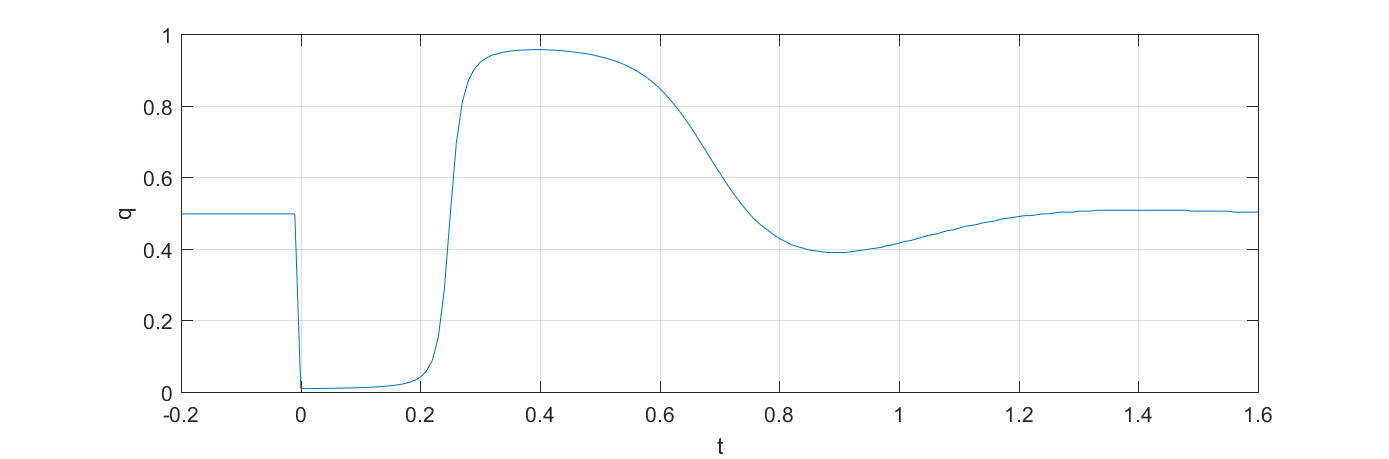
Figure 4: Diversity decay model for $m=5$, $\eta=-10$, $r=5$
Appendix
Derivation of Eq. 1
The equilibrium logistic demand curve for an aggregate load at 50\% duty cycle is given by
\[q = \frac {1} {1+e^{2\eta(1-p)}}.\]where $q$ is the normalized load relative to the maximum load, $\eta$ is the elasticity of demand and $p$ is the normalized price related to the expectation price $\hat P=1$. When the higher-order moments of $P$ are zero, then $\hat P$ is also the most probable price. This function can be represented alternatively by the weighted logistic function
\[q = \frac {\rho_{on} \exp{-2\eta}} {\rho_{on} e^{-2\eta} + \rho_{off} e^{-2\eta p}}\]where the coefficients of the terms in the denominator are $\rho_{off} = \rho_{on} = 0.5$ when the aggregate duty cycle is 50\%. We generalized this from the definition of duty cycle, using $\rho_{on} = D$ and $\rho_{off} = 1-D$ to find
\[Q(p) = \frac {D Q_R} {D + (1-D) e^{2\eta(1-p)} } + Q_U\]or alternatively
\[Q(p) = Q_R \left( 1 + \tfrac{1-D}{D} e^{2\eta(1-p)} \right)^{-1} + Q_U\]with $Q(1) = Q_U + D Q_R$.