Building Load Model Fitting to AMI Data
How to fit a discrete linear-time-invariant dynamic model of building loads to meter data.
There is a great deal of AMI data from individual building meters available to analysts. One problem that I’ve been asked about is how to use AMI data to identify a dynamic model of a building or collection of buildings that we can use in power system studies.
Generally, when we speak of dynamic models we think of linear time-invariant (LTI) models such as continuous time transfer functions, such as those used to relate some input, e.g., outdoor air temperature, to some output of interest, e.g., power demand.
The classical form for these transfer functions is a rational function of the complex frequency $s=\sigma+j\omega$, i.e., $s$-domain, such as
\[\frac{P(s)}{T(s)} = \frac{\beta_{M'}s^{M'}+\cdots+\beta_1s+\beta_0}{\alpha_{N'}s^{N'}+\cdots+\alpha_1s+\alpha_0} \qquad \mathrm{where} ~ N' \ge M'.\]Although such functions are very useful analytically, the discrete LTI forms of these models are much more practical because they can be easily implemented in computer code and controllers that are designed to update at the regular time interval $t_s$. These models are presented in discrete time, e.g., $z$-domain, where $z=e^{st_s}$. Using the bilinear transformation $s \approx \frac{2}{t_s} \frac{z-1}{z+1}$ we obtain a discrete-time transfer function of the form
\[\frac{P(z)}{T(z)} = \frac{b_0+b_1z^{-1}+\cdots+b_Mz^{-M}}{1+a_1z^{-1}+\cdots+a_Nz^{-N}} \qquad \mathrm{where} ~ N \ge M.\]We can rewrite this transfer function as a finite difference equation in discrete time $k$ such that at the time $t=k t_s$
\[P(k) = - a_1 P(k-1) - \cdots - a_N P(k-N) + b_0 T(k) + b_1 T(k-1) + \cdots + b_M T(k-M).\]If we have $K$ samples at the regular interval $t_s$ for $T$ and $P$, then we define the matrix
\[\mathbf{M} = \begin{bmatrix} \mathbf{P}_1 & \cdots & \mathbf{P}_N & \mathbf{T}_0 & \cdots & \mathbf{T}_M \end{bmatrix}\]where
\[\mathbf{T}_k = \begin{bmatrix} T(k) & \cdots & T(K-N+k-1) \end{bmatrix}^\mathrm{T},\] \[\mathbf{P}_k = \begin{bmatrix} P(k) & \cdots & P(K-N+k-1) \end{bmatrix}^\mathrm{T},\]and the vector
\[\mathbf{b} = \begin{bmatrix} P(0) & \cdots & P(K-N-1) \end{bmatrix}^\mathrm{T}.\]We then evaluate $\mathbf{x} = ( \mathbf{M}^T \mathbf{M} )^{-1} \mathbf{M}^T \mathbf{b}$ to obtain the coefficients of the discrete-time transfer function such that
\[\mathbf{x} = \begin{bmatrix} a_1 & \cdots & a_N & b_0 & \cdots & b_M \end{bmatrix}.\]Notice that when there are missing values of $T$ or $P$, it is sufficient to delete the affected rows of $\mathbf{M}$ and $\mathbf{b}$, provided there are sufficient remaining samples such that $K>M+N$. If there are not sufficient samples remaining or there are too many samples of $T$ and $P$ that are too similar, the problem can still be solved for the poorly or under-determined condition, i.e., $\mathbf{x} = \mathbf{M}^T ( \mathbf{M} \mathbf{M}^T )^{-1} \mathbf{b}$. This provides us the least-squares solution as the “best guess” for the fitted model.
Example
The following example uses a building simulation from GridLAB-D which outputs 1 month of building hourly interval energy and outdoor air temperature. First we import the data
import pandas as pd
data = pd.read_csv('data.csv',index_col=['t'],parse_dates=[0])
print(data)
                                 P     T
t
2020-07-01 01:00:00-07:00  3.61584  15.2
2020-07-01 02:00:00-07:00  3.96148  14.2
2020-07-01 03:00:00-07:00  4.60248  13.2
2020-07-01 04:00:00-07:00  5.39665  12.1
2020-07-01 05:00:00-07:00  6.13824  11.1
...                            ...   ...
2020-07-31 20:00:00-07:00  4.82946  16.7
2020-07-31 21:00:00-07:00  4.22882  16.3
2020-07-31 22:00:00-07:00  3.78543  16.0
2020-07-31 23:00:00-07:00  3.59467  15.9
2020-08-01 00:00:00-07:00  3.57846  15.7

[744 rows x 2 columns]
We process the data and solve the model fit problem using a second-order thermal model for the building
X = np.matrix(data['T']).transpose()
Y = np.matrix(data['P']).transpose()
K = 2
L = len(Y)
M = np.hstack([np.hstack([Y[n+1:L-K+n] for n in range(K)]),
               np.hstack([X[n+1:L-K+n] for n in range(K+1)])])
Mt = M.transpose()
x = np.linalg.solve(Mt*M,Mt*Y[K+1:])
From $x$ we extract the polynomial terms for the transfer function’s numerator $b$ and denominator $a$:
a = x.transpose().round(4).tolist()[0][0:K]
a.insert(0,1.0)
b = x.transpose().round(4).tolist()[0][K:]
print(a,b)
[1.0, 0.0067, 0.673] [-0.5364, -1.0575, 1.7641]
Validation
To validate the performance of the model, we use data that was not included in the original dataset.
test = pd.read_csv('test.csv',index_col=['t'],parse_dates=[0])
print(test)
                                 P     T
t
2020-08-01 01:00:00-07:00  3.55169  15.6
2020-08-01 02:00:00-07:00  3.56701  15.4
2020-08-01 03:00:00-07:00  3.66880  15.3
2020-08-01 04:00:00-07:00  3.98450  15.1
2020-08-01 05:00:00-07:00  4.29065  15.0
...                            ...   ...
2020-08-07 20:00:00-07:00  4.73422  16.1
2020-08-07 21:00:00-07:00  4.48835  15.6
2020-08-07 22:00:00-07:00  4.01017  15.0
2020-08-07 23:00:00-07:00  3.87611  14.4
2020-08-08 00:00:00-07:00  3.89687  13.3

[168 rows x 2 columns]
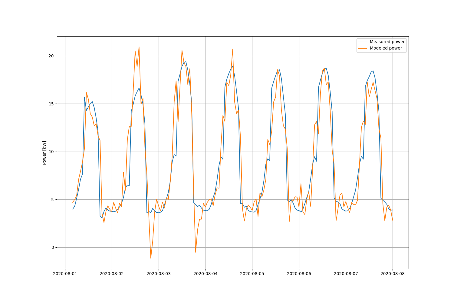
We can use the matrix $M$ for the test data to visualize the performance of the result.
X = np.matrix(test['T']).transpose()
Y = np.matrix(test['P']).transpose()
L = len(Y)
M = np.hstack([np.hstack([Y[n+1:L-K+n] for n in range(K)]),
               np.hstack([X[n+1:L-K+n] for n in range(K+1)])])
plt.figure(figsize=(15,10))
plt.plot(test.index[K+1:],Y[K+1:],label='Measured power')
plt.plot(test.index[K+1:],M@x,label='Modeled power')
plt.grid()
plt.ylabel('Power [kW]')
plt.legend()
plt.show()

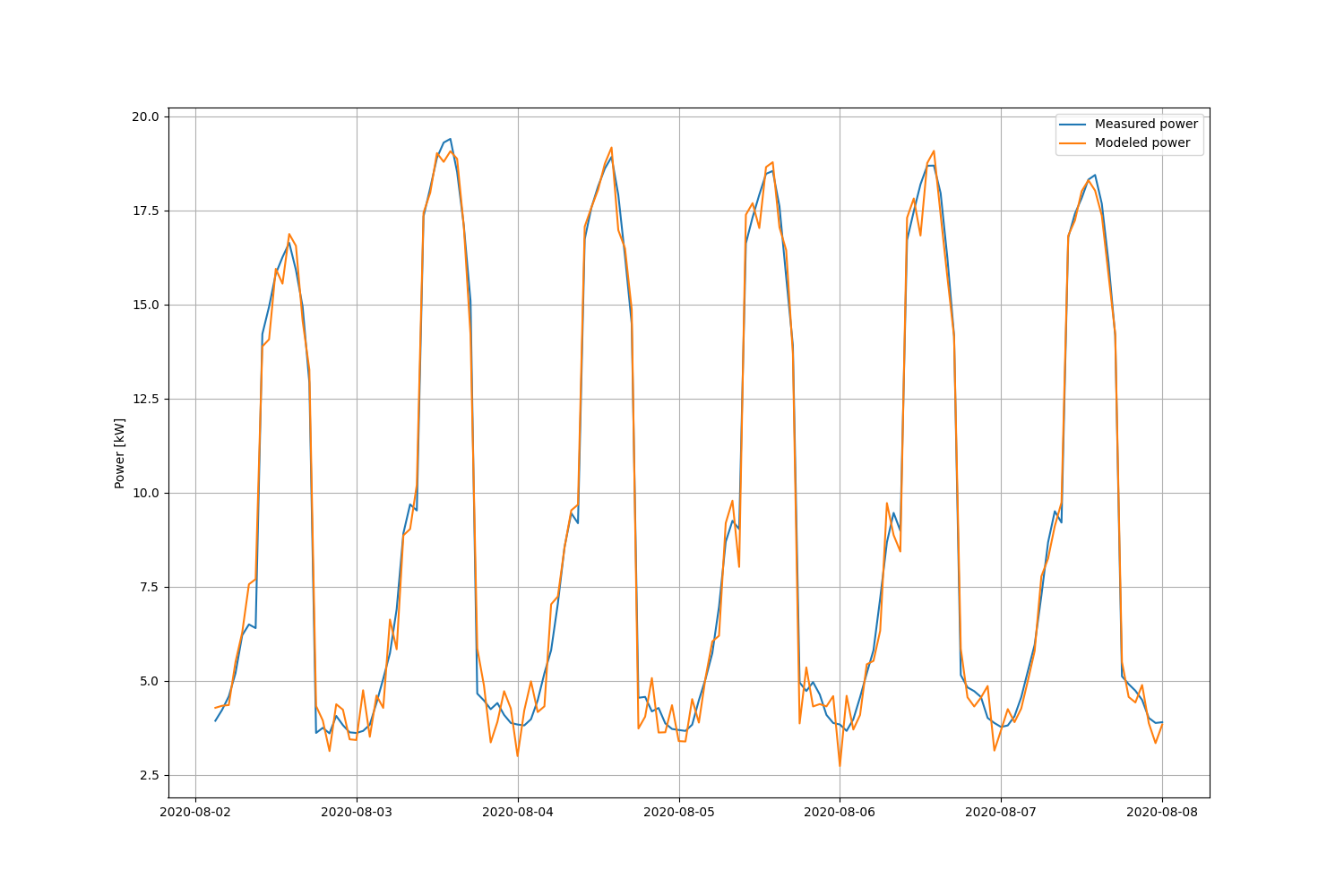
We can see significant errors do appear, particularly during peak and low-load periods. The overall standard error is $\sigma=2.3$ kW. The issue is that the transition from on-peak to off-peak has a highly periodic diurnal component and is very sensitive to small differences during a fast transient event. To remedy this problem we increase the order $K$ of the model to include the last day of data. The result of increasing it to $K=25$ is a significant reduction in the errors. Using the higher-order model, the overall standard error is now $\sigma=0.56$ kW.
